Excel’s Power Query allows you to append several files from a folder using the “Get Data-> From File – > From Folder” option. One of the main requirements to achieve this is that all the files in the folder need to have the same format when it comes to columns, but what happens when some of your files have less columns than the main one?
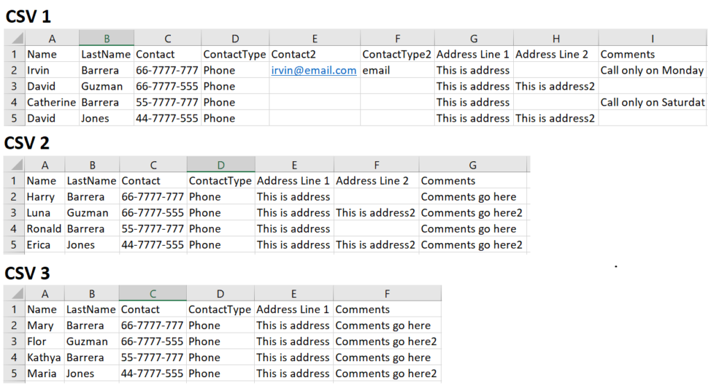
Let’s see how to solve this problem using the below example:

If the data inside your files is formatted as an Excel Table, this shouldn’t be an issue, because Excel will automatically recognize the tables and headers and place them based on the column name and not on position:

However, if you’re dealing with more complex data structures or integrating Power Query with other Microsoft tools, you might need additional expertise. That’s where Microsoft Power Platform consulting services can be useful in optimizing data transformation processes.
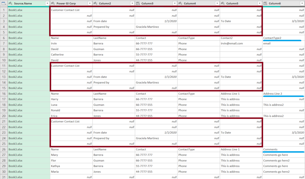
But, if your files are in csv format or if the data is not formatted as a table inside the file, this is how Power Query will place the data:

The files were processed based on position and now we have Contact Type 2, Address Line 2 and Comments under the same column.
The first thought would be to format the data in each of the files as tables, but what if you process 20-50 csv files a day? Nobody wants to manually manipulate 20 different files, let’s better have Power Query do the trick for us!
The solution: Promote Headers in the “Transform Sample File”
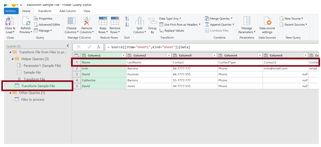
After connecting to a folder, in the queries section, you will see a query called “Transform Sample File”, open it and you will notice that the column names from our files are being set as the first row, and not as actual headers. Let’s set this row as our header.

We do this by using the “Use First Row as Headers” option in the ribbon, after clicking it, you should see the correct column names but there will also be a new step called “Changed Type”, make sure to delete this step from this sample query. (Note: this needs to be removed because this step is applying format to each column based on their name, for example, if the sample file has a “Contact2” column, it will always try to format it in ALL your files, and if your file doesn’t have it, it will error out).
This is how the final sample query should look:

Now, let’s go back to the main query that is combining all the files. You will see an “Expression error” showing up instead of the results, this is because this query is referencing the old column names (Column1, Column2, Column3…), to fix this error, just delete the “Changed Type” step.

After that, you will see how the headers are correctly placed and it’ll show “null” when the column is missing from a source file.

One caveat to this is that the “Sample file” should be a file containing the highest number of columns.
This can also be automated but requires an additional step, we have created an entry on the topic:
https://powergi.net/2020/04/05/power-query-files-from-folder-make-the-sample-file-the-one-with-the-most-columns/
Beyond promoting headers
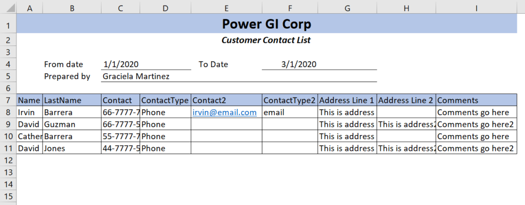
Another scenario where you may want to modify the “Transform sample file” query is when files have some rows on top of the table as a “Document Header”, if your data is not formatted as an excel table, same issue will happen.


The underlying solution for this scenario is the same, you need to modify the “Transform Sample File” query, but adding a couple more basic steps (depending on your specific files). In this specific case, we can remove “null” values in Column4 and that will make all unnecessary records go away.

After removing nulls, promote headers and don’t forget to remove the “Change type” step (Like we did in previous example).
After that, go back to the main query and remove the existing “Change Type” step that is referring to the old column order.

Now, you’re all set, unnecessary records have been removed and the headers are correctly assigned.


